
Read More: Calculus 2 & Calculus 3
1. Limits
Calculus means “a method of calculation or reasoning.” When one computes the sales tax on a purchase, one employs a simple calculus. When one finds the area of a polygonal shape by breaking it up into a set of triangles, one is using another calculus. Proving a theorem in geometry employs yet another calculus.
Despite the wonderful advances in mathematics that had taken place into the first half of the 17th century, mathematicians and scientists were keenly aware of what they could not do. (This is true even today.) In particular, two important concepts eluded mastery by the great thinkers of that me: area and rates of change.
Area seems innocuous enough; areas of circles, rectangles, parallelograms, etc., are standard topics of study for students today just as they were then. However, the areas of arbitrary shapes could not be computed, even if the boundary of the shape could be described exactly.
Rates of change were also important. When an object moves at a constant rate of change, then “distance = rate× me.” But what if the rate is not constant – can distance s ll be computed? Or, if distance is known, can we discover the rate of change?
It turns out that these two concepts were related. Two mathematicians, Sir Isaac Newton and Gottfried Leibniz, are credited with independently formulating a system of computing that solved the above problems and showed how they were connected. Their system of reasoning was “a” calculus. However, as the power and importance of their discovery took hold, it became known to many as “the” calculus. Today, we generally shorten this to discuss “calculus.”
The foundation of “the calculus” is the limit. It is a tool to describe a particular behavior of a function. This chapter begins our study of the limit by approximating its value graphically and numerically. After a formal definition of the limit, properties are established that make “finding limits” tractable. Once the limit is understood, then the problems of area and rates of change can be approached.
An Introduction To Limits
We begin our study of limits by considering examples that demonstrate key concepts that will be explained as we progress.
Consider the function![]() When x is near the value 1, what value (if any) is y near? While our ques on is not precisely formed (what constitutes “near the value 1”?), the answer does not seem difficult to find. One might think first to look at a graph of this function to approximate the appropriate y values. Consider Figure 1.1.1, where
When x is near the value 1, what value (if any) is y near? While our ques on is not precisely formed (what constitutes “near the value 1”?), the answer does not seem difficult to find. One might think first to look at a graph of this function to approximate the appropriate y values. Consider Figure 1.1.1, where ![]() is graphed. For values of x near 1, it seems that y takes on values near 0.85. In fact, when x = 1, then y = sin 1
is graphed. For values of x near 1, it seems that y takes on values near 0.85. In fact, when x = 1, then y = sin 1
1 ≈ 0.84, so it makes sense that when x is “near” 1, y will be “near” 0.84.
Consider this again at a different value for x. When x is near 0, what value (if any) is y near? By considering Figure 1.1.2, one can see that it seems that y takes on values near 1. But what happens when x = 0? We have
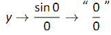
The expression “0/0” has no value; it is indeterminate. Such an expression gives no information about what is going on with the function nearby. We cannot find out how y behaves near x = 0 for this function simply by le ng x = 0.
Finding a limit entails understanding how a function behaves near a par cu- lar value of x. Before continuing, it will be useful to establish some nota on. Let y = f(x); that is, let y be a function of x for some function f. The expression “the limit of y as x approaches 1” describes a number, often referred to as L, that y nears as x nears 1. We write all this as
This is not a complete definition (that will come in the next sec on); this is a pseudo-definition that will allow us to explore the idea of a limit.
Above, where f(x) = sin(x)/x, we approximated
![]()
(We approximated these limits, hence used the “≈” symbol, since we are working with the pseudo-definition of a limit, not the actual definition.)
Once we have the true definition of a limit, we will find limits analytically; that is, exactly using a variety of mathematical tools. For now, we will approximate limits both graphically and numerically. Graphing a function can provide a good approximation, though often not very precise. Numerical methods can provide a more accurate approximation. We have already approximated limits graphically, so we now turn our attention to numerical approximations.


